
By Gabriel Vasconcelos
When the LASSO fails?
The LASSO has two important uses, the first is forecasting and the second is variable selection. We are going to talk about the second. The variable selection objective is to recover the correct set of variables that generate the data or at least the best approximation given the candidate variables. The LASSO has attracted a lot of attention lately because it allows us to estimate a linear regression with thousands of variables and the model select the right ones for us. However, what many people ignore is when the LASSO fails.
Like any model, the LASSO also rely on assumptions in order to work. The first is sparsity, i.e. only a small number of variables may actually be relevant. If this assumption does not hold there is no hope to use the LASSO for variable selection. Another assumption is that the irrepresentable condition must hold, this condition may look very technical but it only says that the relevant variable may not be very correlated with the irrelevant variables.
Suppose your candidate variables are represented by the matrix 


The first piece, 


The inequality above must hold for all elements. 


Example
For this example we are going to generate two covariance matrices, one that satisfies the irrepresentable condition and one that violates it. Our design will be very simple: only 10 candidate variables where five of them are relevant.
library(mvtnorm)
library(corrplot)
library(glmnet)
library(clusterGeneration)
k=10 # = Number of Candidate Variables
p=5 # = Number of Relevant Variables
N=500 # = Number of observations
betas=(-1)^(1:p) # = Values for beta
set.seed(12345) # = Seed for replication
sigma1=genPositiveDefMat(k,"unifcorrmat")$Sigma # = Sigma1 violates the irc
sigma2=sigma1 # = Sigma2 satisfies the irc
sigma2[(p+1):k,1:p]=0
sigma2[1:p,(p+1):k]=0

# = Verify the irrepresentable condition
irc1=sort(abs(sigma1[(p+1):k,1:p]%*%solve(sigma1[1:p,1:p])%*%sign(betas)))
irc2=sort(abs(sigma2[(p+1):k,1:p]%*%solve(sigma2[1:p,1:p])%*%sign(betas)))
c(max(irc1),max(irc2))
## [1] 3.222599 0.000000
# = Have a look at the correlation matrices
par(mfrow=c(1,2))
corrplot(cov2cor(sigma1))
corrplot(cov2cor(sigma2))

As you can see, irc1 violates the irrepresentable condition and irc2 does not. The correlation matrix that satisfies the irrepresentable condition is block diagonal and the relevant variables have no correlation with the irrelevant ones. This is an extreme case, you may have a small correlation and still satisfy the condition.
Now let us check how the LASSO works for both covariance matrices. First we need do understand what is the regularization path. The LASSO objective function penalizes the size of the coefficients and this penalization is controlled by a hyper-parameter 

X1=rmvnorm(N,sigma = sigma1) # = Variables for the design that violates the IRC = #
X2=rmvnorm(N,sigma = sigma2) # = Variables for the design that satisfies the IRC = #
e=rnorm(N) # = Error = #
y1=X1[,1:p]%*%betas+e # = Generate y for design 1 = #
y2=X2[,1:p]%*%betas+e # = Generate y for design 2 = #

lasso1=glmnet(X1,y1,nlambda = 100) # = Estimation for design 1 = #
lasso2=glmnet(X2,y2,nlambda = 100) # = Estimation for design 2 = #

## == Regularization path == ##
par(mfrow=c(1,2))
l1=log(lasso1$lambda)
matplot(as.matrix(l1),t(coef(lasso1)[-1,]),type="l",lty=1,col=c(rep(1,9),2),ylab="coef",xlab="log(lambda)",main="Violates IRC")
l2=log(lasso2$lambda)
matplot(as.matrix(l2),t(coef(lasso2)[-1,]),type="l",lty=1,col=c(rep(1,9),2),ylab="coef",xlab="log(lambda)",main="Satisfies IRC")

The plot on the left shows the results when the irrepresentable condition is violated and the plot on the right is the case when it is satisfied. The five black lines that slowly converge to zero are the five relevant variables and the red line is an irrelevant variable. As you can see, when the IRC is satisfied all relevant variables shrink very fast to zero as we increase lambda. However, when the IRC is violated one irrelevant variable starts with a very small coefficient that slowly increases before decreasing to zero in the very end of the path. This variable is selected through the entire path, it is virtually impossible to recover the correct set of variables in this case unless you apply a different penalty to each variable. This is precisely what the adaptive LASSO does. Does that mean that the adaLASSO is free from the irrepresentable condition??? The answer is: partially. The adaptive LASSO requires a less restrictive condition called weighted irrepresentable condition, which is much easier to satisfy. The two plots below show the regularization path for the LASSO and the adaLASSO in the case the IRC is violated. As you can see, the adaLASSO selects the correct set of variables in all the path.
lasso1.1=cv.glmnet(X1,y1)
w.=(abs(coef(lasso1.1)[-1])+1/N)^(-1)
adalasso1=glmnet(X1,y1,penalty.factor = w.)

par(mfrow=c(1,2))
l1=log(lasso1$lambda)
matplot(as.matrix(l1),t(coef(lasso1)[-1,]),type="l",lty=1,col=c(rep(1,9),2),ylab="coef",xlab="log(lambda)",main="LASSO")
l2=log(adalasso1$lambda)
matplot(as.matrix(l2),t(coef(adalasso1)[-1,]),type="l",lty=1,col=c(rep(1,9),2),ylab="coef",xlab="log(lambda)",main="adaLASSO")

The biggest problem is that the irrepresentable condition and its less restricted weighted version are not testable in the real world because we need the populational covariance matrix and the true betas that generate the data. The solution is to study your data as much as possible to at least have an idea of the situation.
Some articles on the topic
Zhao, Peng, and Bin Yu. “On model selection consistency of Lasso.” Journal of Machine learning research 7.Nov (2006): 2541-2563.
Meinshausen, Nicolai, and Bin Yu. “Lasso-type recovery of sparse representations for high-dimensional data.” The Annals of Statistics (2009): 246-270.

Amazing, I finally get the problems often forgotten of Lasso
LikeLike
Pingback: When the LASSO fails??? | A bunch of data
Pingback: When the LASSO fails??? – Mubashir Qasim
Hi.
Does elastic-net suffer from the same problem?
What other alternatives do we have?
LikeLike
I don’t know the exact condition for the elastic-net. But its penalization is less restrictive than the LASSO in a way that it normally selects more variables. It probably has a similar problem. The adaptive versions are the best you can get as far as I know.
LikeLike
The elastinet is a linear combination of ridge and lasso. Unless your elastinet says that straight lasso is best, it will contain some ridge and will not remove coefficients. I can expand on this if you like.
LikeLike
Yes. But it also needs a condition called elastic irrepresentable condition to have model selection consistency. It is more complicated because you also need to know the values of lambda for both the l1 and the l2 norm.
LikeLike
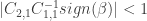
What do you mean by |C_{21}C_{11}^{-1} sign(|beta)| < 1 in particular what does “|” mean. Is it a norm ? The C are matrices and can be multiplied, but do you want to take their determinant and then ordinary absolute value or is this a norm like Frobenius ?
LikeLike
This formula will return a vector. It has to be smaller than one element-wise. | stands for absolute value.
LikeLike
“return a vector” , you mean consider the resultant matrix as a vector ? So the norm is max of absolute value of the components ?
LikeLike
No. I mean it is a vector because sign(beta) is a vector. But you are right, we are interested in the maximum absolute value of the components.
LikeLike
Pingback: Distilled News | Data Analytics & R
Hi, thanks for this post. Maybe I overlooked it, but in the formulas beta is used before it is defined and in the code it is set at betas=(-1)^(1:p) # = Values for beta and then below there is the criterion. What does beta stand for? Thank you!
LikeLike
These betas defined in the code are the real betas used to generate the data. The irrepresentable condition is not testable because you need to know these betas. Since in this case I generate the data, I know exactly the true betas but this is not true if you are working with real data.
LikeLike
Thank you for this article !
How do you define “relevant” and “irrelevant” variables ?
Are relevant variables those selected at the end by the model ? Or those that you think are important before running the LASSO selection ?
LikeLike
Relevant variables are the ones I use to generate y in the code. In this case, the first five variables are relevant.
LikeLike
And in “real world” analysis? How do you know which explicative variables are relevant and which ones are not?
LikeLike
You don’t. But you have an idea on how correlated your variables are and if the lasso might work or not. If the condition is satisfied you will recover the correct set of variables with high probability. If it fails you will probably still recover the correct set of variables plus some irrelevants.
LikeLike
Ok, so actually the collinearity is an issue for variable selection with LASSO (and I guess elactic net too). I was adviced to use this kind of variable selection because of high colinearity in my dataset and being able to have an “automatic” variable selection, instead of manually select variable in relation to a threshold of correlation between explicative variables. But first results were quite disapointing. In particular, two highly correlated variables were selected, but one had a negative coefficient while it showed a positive relationship with the response variable…
LikeLike
Collinearity between relevants and irrelevants yes. Try the adaLASSO to increase your chances because the condition is less restrictive.
LikeLike
I will! Thank you!
LikeLike
Pingback: Machine Learning for Beginners, Part 12: Lasso – The Data Lass